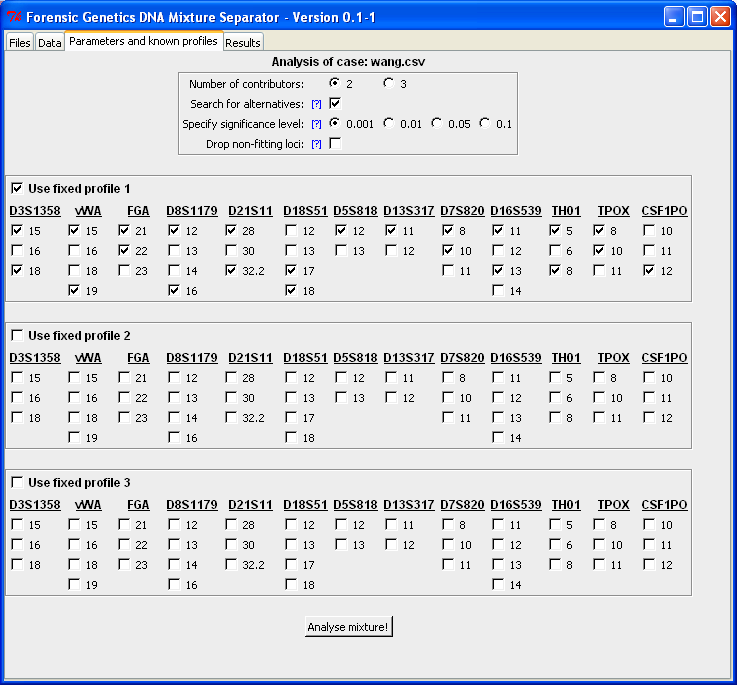
The "Parameters and known profiles"-tab makes it possible to specify the number of contributors, whether the algorithm should search for alternatives and fixed/known profiles. We assume the sample is a two-person mixture and searches for alternatives (the lower the level of significance is, the more alternatives are included in the final result). Furthermore, we want to investigate whether the profile in Table 1 is a possible contributor to the DNA mixture.
| Locus | D3 | vWA | FGA | D8 | D21 | D18 | D5 | D13 | D7 | D16 | TH01 | TPOX | CFS |
|---|---|---|---|---|---|---|---|---|---|---|---|---|---|
| True offender | 15 18 | 15 19 | 21 22 | 12 16 | 28 32.2 | 17 18 | 12 12 | 11 12 | 8 10 | 11 13 | 5 6 | 8 10 | 11 12 |
| Suspect | 15 18 | 15 19 | 21 22 | 12 16 | 28 32.2 | 17 18 | 12 12 | 11 11 | 8 10 | 11 13 | 5 8 | 8 10 | 12 12 |
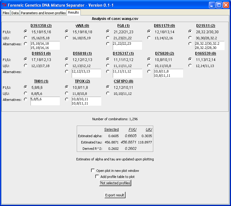
When clicking "Analyse mixture!" the computer resolves the DNA mixture and returns result in the "Result"-tab. Below is the output from the analysis. For each locus the unknown profile that together with the fixed profile best explains the DNA mixture is identified (denoted "F1/U" for "Fixed profile 1" and "Unknown"). In the row below ("U/U") is the best matching configurations (both profiles unspecified, i.e. "U/U" is short for "Unknown/Unknown"). Furthermore, below is a list of possible alternative configurations including the fixed profile.
Next to the locus designation is the number of possible alternatives for that locus given in parenthesis. Below the list of locus configurations is the number of total configurations given together with the estimated parameters of the statistical model. The "Estimated alpha" for "F1/U" represents the mixture proportion of the fixed contributor, whereas for "U/U" it denotes the contribution from the minor contributor. Here alpha is respectively 0.66 and 0.3, which approximately corresponds to an 1:2-mixture ratio in both cases. The "Estimated tau" value represents that residual variance, which means that the smaller the estimate the better is the concordance between the observed and expected peak intensities. The "Derived R^2" is computed as the tau for "U/U" to tau for "F1/U". Here R^2 = 0.26 = 118/457 implying that the residual variance is four times bigger when the suspect's profile is assumed in the mixture compared to the best matching pair (which is identical to the true contributors, see best matching guide):
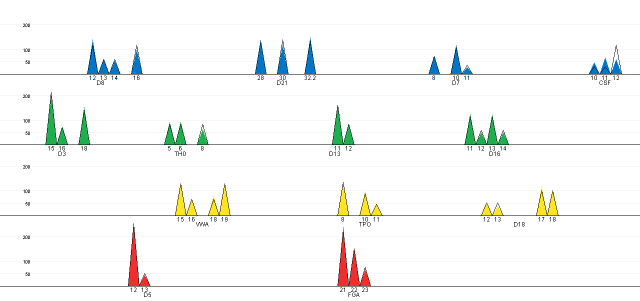
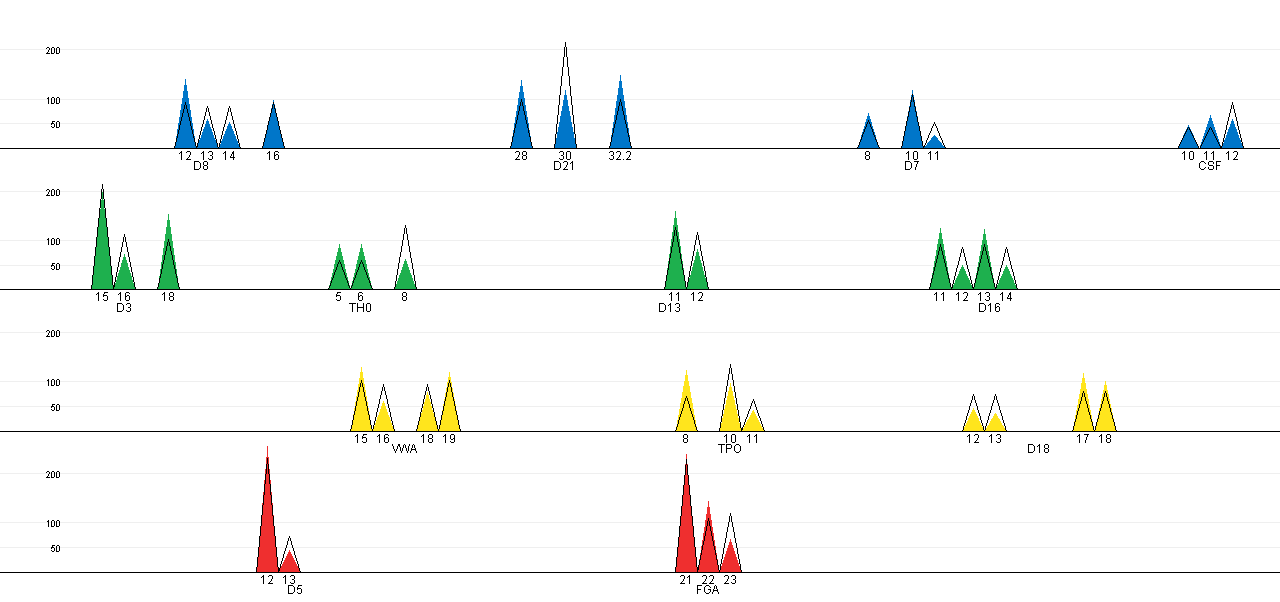
The expected peak intensities for the selected configuration can be
plotted against the observed peak intensities in a EPG-like plot. The
coloured cones represents the observed peak intensities, while the
black lined cones show the expected peak intensities. Note that the
configuration on CSF causes the expected peak intensities to deviate
from the observed. This is also the only combination of the three
changes between the true offender and suspect (see Table 1), that is not among the alternatives in the
best matching analysis (see results of
best matching analysis - where it should be remembered that the
suspect corresponds to the major profile).
From the analysis output alternative configurations can be specified by marking the combinations in the lists. For each locus the list of alternatives is sorted in decreasing order in terms of goodness-of-fit. For the selected configuration the "R^2" quantity is computed as the ratio of the estimated tau values of the best matching ("U/U") and the selected configuration. Here R^2 = 0.06 = 118/2055 and the closer R^2 is to 1, the better is the alternative configuration relative to the best match pair of profiles:
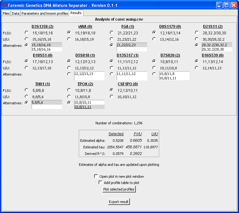
In the plot below we see a change in the fit between the black lined
cones and coloured cones. The low value of R^2 is indicates a poor fit
between the observed and expected peak intensities, which is pictured
below. In addition to the plot it is possible to export the results to
a ASCII text file by clicking "Export results". For this example the
text file is: wang_result-suspectalternative.txt
References
Wang T, N Xue and JD Birdwell (2006). 'Least-Square Deconvolution: A
Framework for Interpreting Short Tandem Repeat Mixtures'. Journal of
Forensic Science 51 (6): 1284-1297. DOI: 10.1111/j.1556-4029.2006.00268.x