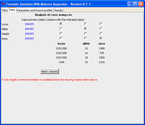
By marking the file name and click the "Analyse file"-button (or double-click on the file name), we obtain the "Data"-tab shown below. In the "Data"-tab the columns containing the relevant information are selected. Since wang.csv only contain information about locus, allele and area, we leave "Height" empty:
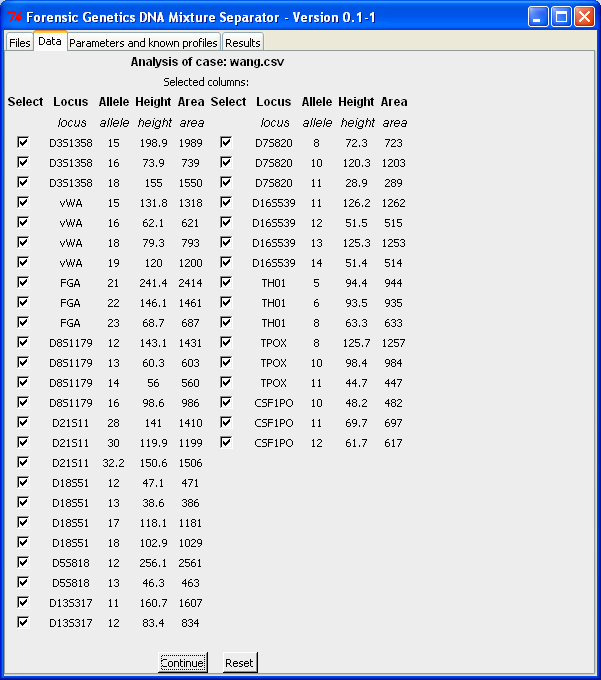
After the columns are selected (by clicking "Select columns"), we obtain all the rows (for the selected columns) in the file. For each row it is possible to select/remove the peak from the analysis. However, we recommend that the removal of rows is used with caution, since all information should be considered and dealt with!
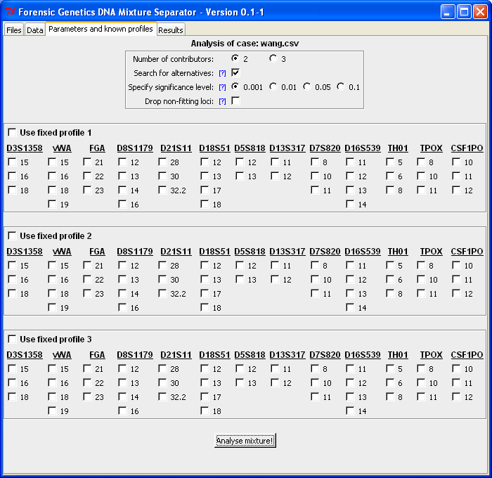
The "Parameters and known profiles"-tab makes it possible to specify the number of contributors, whether the algorithm should search for alternatives, etc. It is also here that fixed/known profiles can be specified (see the Fixed profile analysis guide for more details). We assume the sample is a two-person mixture and searches for alternatives (the lower the level of significance is, the more alternatives are included in the final result):
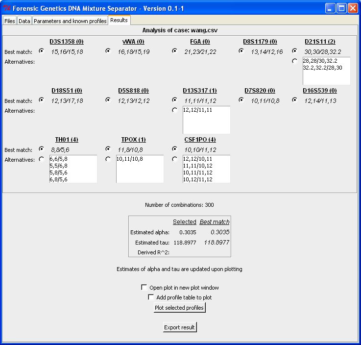
When clicking "Analyse mixture!" the computer resolves the DNA mixture and returns result in the "Result"-tab. Below is the output from the analysis. For each locus a best matching configuration (which is identical to the true profiles, see by Wang et al., 2006) is identified together with a list of possible alternatives. Next to the locus designation is the number of possible alternatives for that locus given in parenthesis. Below the list of locus configurations is the number of total configurations given together with the estimated parameters of the statistical model. The "Estimated alpha" represents the mixture proportion of the minor contributor. Here it is 0.3 which corresponds to an 1:2-mixture ratio. The "Estimated tau" value represents that residual variance, which means that the smaller the estimate the better is the concordance between the observed and expected peak intensities (the "Derived R^2" quantity is explained below):
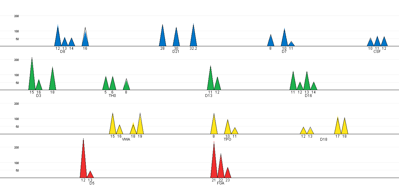
The expected peak intensities for the selected configuration can be
plotted against the observed peak intensities in a EPG-like plot. The
coloured cones represents the observed peak intensities, while the
black lined cones show the expected peak intensities (for this
particular plot it is hard to see any discrepancies, which indicate a
good fit between the observed and expected peak intensities):
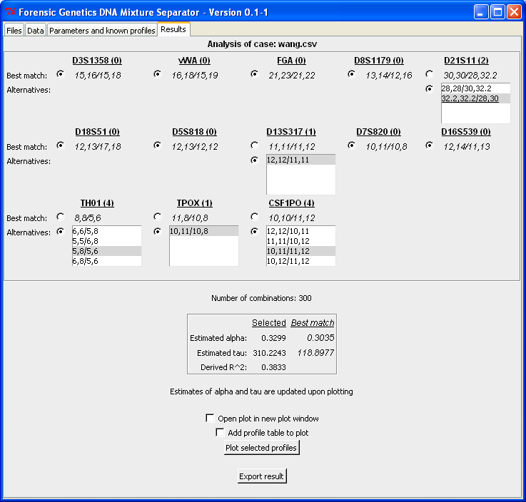
From the analysis output alternative configurations can be specified by marking the combinations in the lists. For each locus the list of alternatives is sorted in decreasing order in terms of goodness-of-fit. For the selected configuration the "R^2" quantity is computed as the ratio of the estimated tau values. Here R^2 = 0.38 = 118/310 and the closer R^2 is to 1, the better is the alternative configuration relative to the best match pair of profiles:
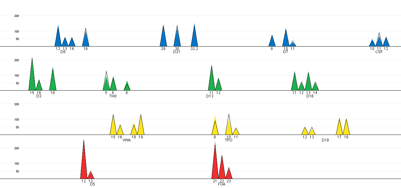
In the plot below we see a change in the fit between the black lined
cones and coloured cones. In addition to the plot it is possible to
export the results to a ASCII text file by clicking "Export
results". For this example the text file is: wang_result-alternative.txt
References
Wang T, N Xue and JD Birdwell (2006). 'Least-Square Deconvolution: A
Framework for Interpreting Short Tandem Repeat Mixtures'. Journal of
Forensic Science 51 (6): 1284-1297. DOI: 10.1111/j.1556-4029.2006.00268.x